
15(20)
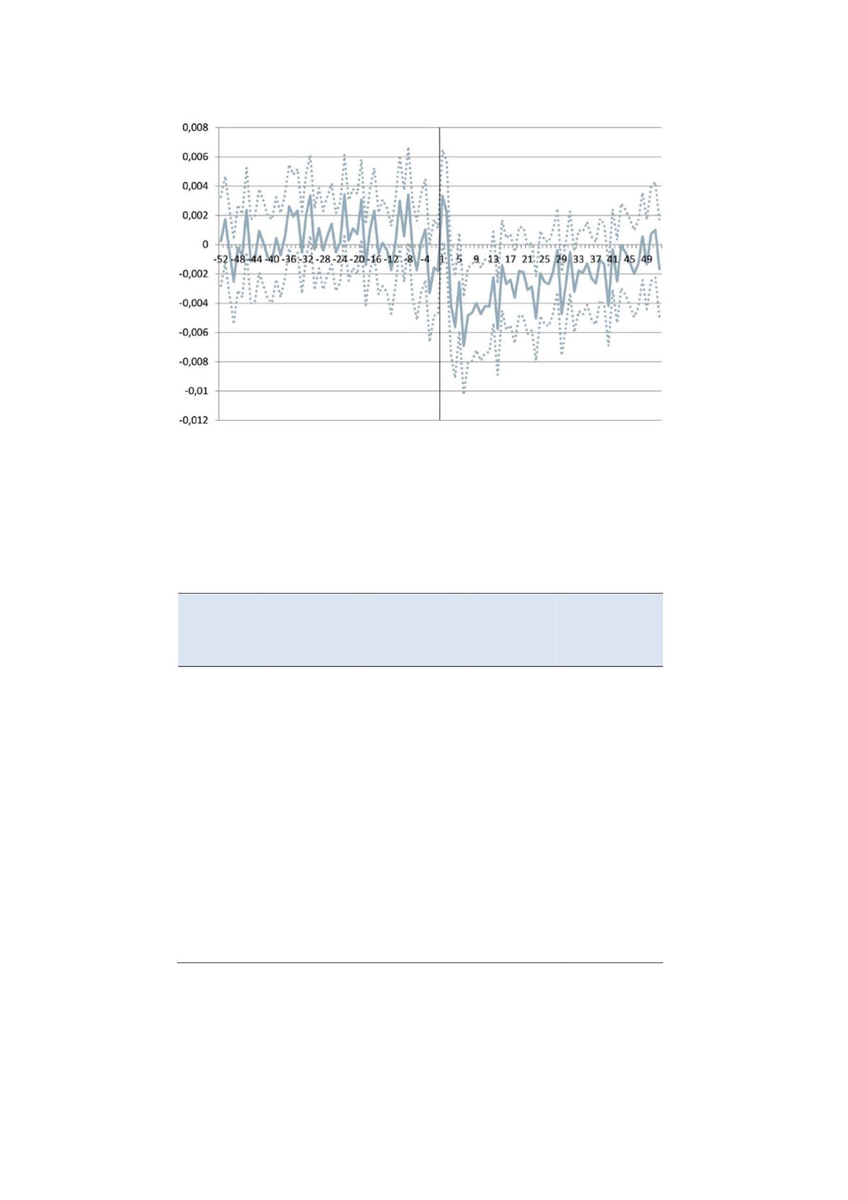
Figure 2.
The effect of monitoring on weekly gross benefit days
Note: The solid line shows the estimated weekly difference in gross benefit days
between the treatment and the comparison group. Randomization to the comparison
group has been done on a weekly basis. The dotted lines show the estimated 95 per
cent confidence interval. Standard errors are robust against heteroskedasticity and
clustered on the parent. The vertical line shows the timing of the treatment
assignment.
Table 2.
The deterrence effect one year after assignment
Effect of
monitoring
(gross benefit
days)
Effect of
monitoring
(per cent)
Number of
parents in the
treatment
group
Number of
parents in the
comparison
group
All parents
–0,127***
(0,027)
–1,4***
313,908
632,817
All, controls
for parent’s
background
–0,126***
(0,026)
–1,2***
311,931
628,776
Mothers
–0,131***
(0,036)
–1,3***
200,066
403,561
Fathers
–0,121***
(0,038)
–1,6***
113,842
229,256
Basic
education
–0,481***
(0,156)
–4,3***
17,534
35,750
Upper-
secondary
education
–0,173***
(0,043)
–1,8***
140,548
283,962
Post-
secondary
education
–0,043
(0,034)
–0,5
155,272
311,967
Note: The effect is estimated with differences-in-differences model. Benefit days
are measured during one year before and after the treatment assignment. Robust
standard errors in parentheses. The model controlling for the parent’s background
include gender, polynomial of income, age, age of the youngest child, number of
children, education level, marital status, born abroad and county. *** p<0.01, **
p<0.05, * p<0.1.


